PLEASE SEND ME E-MAIL IMMEDIATELY IF YOU HAVE PROBLEMS WITH THIS SOFTWARE.
You can start jser from the command-line:
lnx1% jser &Note, that we start jser in the background so that we can continue to type commands at the shell prompt. Also note that jser is an X-application, so even though it is being run on lnx1, the windows should appear on your local screen.
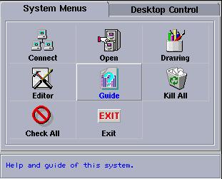
After invocation of jser, the following window should pop up on your screen in a few seconds (but be patient, it may be 15 seconds, or so):

Note that, with the exception of the Exit button---which shuts the server down---you will probably find little use for the various selections on the server panel. Rather, you will primarily interact with the server through additional windows which display data sets which are sent to the server after it is started. For example, assume that we have previously generated an .sdf file using, for example, a Fortran program which calls vsxynt:
   lnx1% pwd
   /usr/people/phys410/fd/new_wave

   lnx1% ls
   Makefile   gpwave.f   vswave.f

   lnx1% make vswave
   f77 -g -64 -c vswave.f
   f77 -g -64 -L/usr/local/lib vswave.o -lp410f -lsvs -lrnpl -lsv -o vswave

   lnx1% vswave
    usage: vswave

   lnx1% vswave 101

   lnx1% ls *.sdf
   wave.sdf
Then, once we have started the scivis server, we can send
the data in this .sdf file to the server using the
sdftosv command:
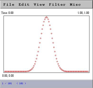
lnx1% sdftosv waveIn a few seconds you should see a window such as the following pop-up:

Observe that the new window displays one time step (dataset) of the data at a time. Using the pull down menus and/or keyboard accelerators, you can step through the data, zoom-in or or, play (animate) the data, and perform many other functions, many of which are fairly self-explanatory.
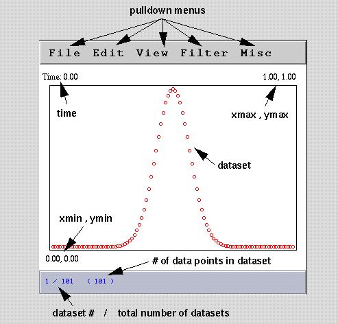
Here is a guide to the annotations on the above scivis data window:

Note that the server's main function (in the context of this course) is to provide you with a useful tool to develop and analyze programs which solve time-dependent partial differential equations in one spatial dimension (or time dependent particle motion in 2 dimensions). In particular, you should not expect to use it to produce ``quality'' hardcopy output.
scivis (jser) keyboard-accelerators
Important Note: Due to a bug in the scivis software, you must first RESIZE any window that scivis creates in order for the following keyboard accelerators to work. All accelerators are Ctrl-key based; for example, C-a means depress the ctrl key and then the a key (without releasing the ctrl key).
| Keystroke | Mnemonic | Function |
|---|---|---|
| C-q | Quit | Closes window |
| C-a | Animate | Starts animation |
| C-s | Stop | Stops animation |
| C-n | Next | Displays next dataset |
| C-p | Previous | Displays previous dataset |
| C-g | Goto | Goto specific dataset |
sdftosv: Sends data in .sdf files to the Scivis server (also known as jser). Here is the full usage for the command
   % sdftosv
sdftosv version: 1.0
  Copyright (c) 1997 by Robert L. Marsa
  sends .sdf files to the scivis visualization server
Usage:
  sdftosv [ -i ivec ]
          [ -n oname ]
          [ -s ]
          input_file [ input_file [ ... ] ]

  -i ivec  -- use ivec (0 based) for output control
  -n oname -- name all data sets oname
  -s       -- send data sets one at a time
              useful for large or nonuniform data
  input_file is an .sdf file
Beware that there is a command sdftovs which sends
an .sdf file to a different server---if you get an
error message such as
  assign_Server: Could not communicate with sgi1
  assign_Server: Ensure that server is running on sgi1 and/or
  assign_Server: check/reset value of environment variable VSHOST.
you have typed sdftovs instead of sdftosv.
A typical invocation will be:
   % ls
   wave.sdf

   % sdftosv wave
Note that you do not have to specify the .sdf extension explicitly, but you can if you so wish.
% sdftosv -i '0-*/2' waveIn this example, the construct
0-*/2is an example of an index-vector (or ivec), which is just a shorthand for a regular sequence of integers:
min-max/step ===> min, min + step, min + 2 step, ... min + n stepwhere n is the largest integer such that
min + n step <= maxIndex 0 refers to the first time level of data stored in the file, and an asterisk (*) can be used in place of min and/or max to denote "first time-level" or "last time-level" respectively. When using * in an index-vector specfication, such as in the above example, be sure to enclose the index-vector in single quotes to keep the shell from interpreting * in its own special way.
IMPORTANT NOTE: The utilities sdftosv and jv1 need to know on which machine jser is running. Often this will be the same machine from which you are sending data, but it need not be so. Thus the utilities require that the environment variable JSERHOST be set to the name of the host which is running jser. On the lnx machines, JSERHOST will be automatically set at shell start-up to the name of the local host, so normally, you won't have to worry about setting it explicitly. However, if you want to send data from some other machine, say physics.ubc.ca, to jser running on lnx1, for example, then on physics you will need to issue:
physics% setenv JSERHOST lnx1before you transmit the data.
sdfinfo: Program which dumps summary information about an .sdf to standard output.
Typical usage:
   % sdfinfo wave.sdf

   Data set 1
   name=<wave>
   version=1
   time=0
   rank=1
   shape=(10)
   bbox=(0,1)
   csize=10
   dsize=10
   cnames=(r)
   tag=<NULL>
   |data|=0.329628, min(data)=1.38879e-11, max(data)=0.734444
   Data set 2
   name=<wave>
   version=1
   time=0.111111
   rank=1
   shape=(10)
   bbox=(0,1)
   csize=10
   dsize=10
   cnames=(r)
      .
      .
      .
Key to output:
jv1: Filter which reads two columns of numbers
((x,y) pairs) from standard input and then sends the data to
scivis (jser).
Typical usage:
% jv1 < data_fileor
% jv1 name < data_filewhere data_file is a two column file containing the data to plot. In the first instance, the data will be visualized in a jser window named Standard input, in the second the jser window will be labelled name.
libbbhutil.a: Fortran- and C-callable output utility routines written for the Binary Black Holes Grand Challenge Project. Available on lnx machines. Postscript ``man-style'' documentation for the C routines is available here. Fortran routines have the same names (gft_out_bbox etc.) and can be either calledor invoked as integer functions. For output of 2- and 3-D arrays on uniform finite-difference meshes, the routines
gft_out_bbox
should suffice. Here is a usage example:
      integer      nx,        ny
      parameter  ( nx = 65,   ny = 33 )

      real*8       gfcn(nx,ny)
      real*8       xmin,      xmax,     ymin,     ymax,
     &             time

      integer      shape(2),  rank
      real*8       bbox(4)
               .
               .
               .
c------------------------------------------------------
c     'bbox' defines 'bounding box' of coords.
c     associated with the data:
c
c     bbox := ( xmin, xmax, ymin, ymax )
c------------------------------------------------------
      bbox(1) = xmin
      bbox(2) = xmax
      bbox(3) = ymin
      bbox(4) = ymax

      rank = 2
      shape(1) = nx
      shape(2) = ny

      do it = 1 , nt
              .
              .
              .
c------------------------------------------------------
c     The first (string) arg. to 'gft_out_bbox'
c     is stripped of non alphanumeric/underscore
c     characters (including punctuation) if necessary,
c     and then used as the 'stem' for a filename of
c     the form 'stem.sdf'.  All calls to 'gft_out_bbox'
c     with the same string result in output to the
c     same file.
c------------------------------------------------------
         time = it * 1.0d0
         call gft_out_bbox('gfcn',time,shape,rank,
     &                      bbox,gfcn)
      end do
              .
              .
              .